Leading vs Lagging Voice Agent Metrics: Catch Problems Hours Before CSAT Drops
On this page
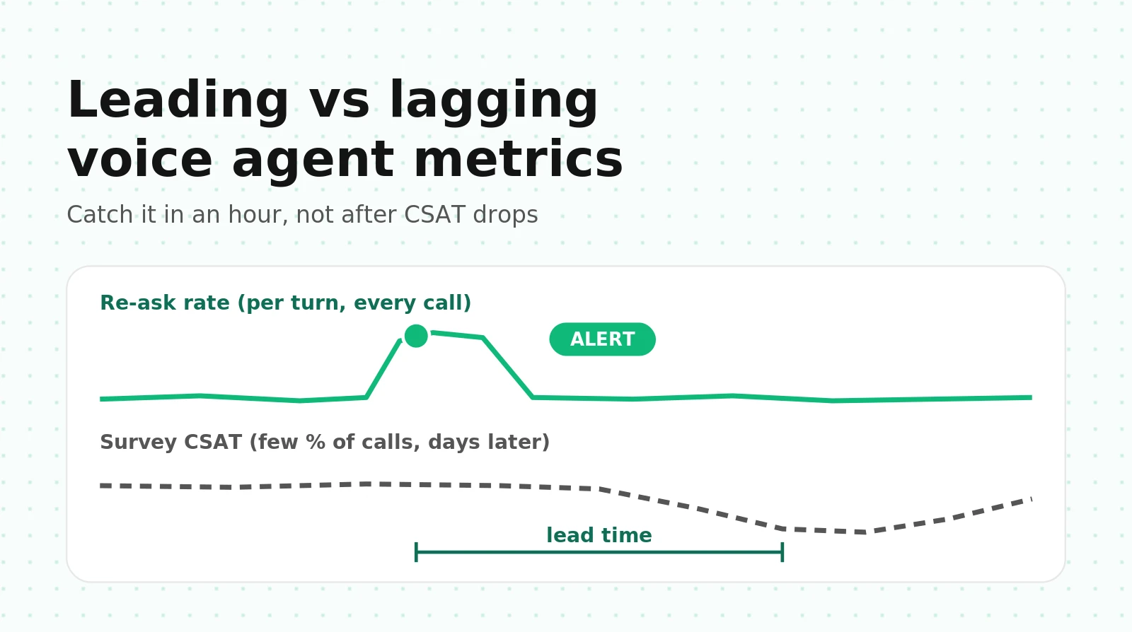
You ship a prompt change on Monday morning. Survey CSAT looks normal Monday night, a little soft Tuesday, and clearly down by Wednesday. By the time someone opens the weekly review, roughly a week of callers has hit the regression. The signal was in your logs within the first hour. You were watching the wrong metrics on the wrong clock.
This guide is about that clock. It puts 15 voice agent metrics on one axis, time-to-signal, and shows how to prove that a fast metric predicts a slow one. It also covers alert design, a worked regression, and pandas code for your own call table. It assumes you already know what you are optimizing (if not, start with the north-star metric) and that you log turn-level events (see what to log on every call).
What leading vs lagging indicators mean for a voice agent
The textbook definition says a leading indicator moves before the outcome and a lagging indicator confirms it afterward. That is too vague to act on. For a voice agent, two concrete properties separate them.
Time-to-signal. This is how long after a change you can tell, with statistical confidence, that the metric moved. It has three parts:
`time_to_signal = emit_delay + pipeline_delay + accumulation_time`
- Emit delay: how long after the call the value exists. Turn latency exists the moment the turn ends. A survey answer exists when the caller bothers to reply. "Called back within 7 days" exists only after 7 days.
- Pipeline delay: batch jobs, CRM syncs, warehouse loads. Often hours for anything that touches a ticketing or billing system.
- Accumulation time: how long you need to collect enough observations to separate a real shift from noise. `accumulation_time = n_required / observations_per_hour`.
The third term usually dominates, and it is where data availability comes in.
Observations per call. Re-ask rate, interruption rate and turn latency produce several observations on every call, one per turn. Containment and handle time produce one per call. CSAT produces one per surveyed and answering call, which is a small fraction. Churn produces one per customer per billing period. A metric with 8 observations per call and 100% coverage accumulates evidence roughly 100 times faster than one with 1 observation on 8% of calls.
So a working definition:
- Leading indicator: a metric readable within minutes to hours of a change, measured on every call, and shown to predict a lagging outcome you care about.
- Lagging indicator: an outcome metric you care about directly, readable only after days or weeks, often on a subset of calls.
The word "shown" is the part most teams skip. A fast metric that predicts nothing is just a fast metric.
The map: 15 voice agent metrics by time-to-signal
The table below sorts common voice agent KPIs from fastest to slowest. The time-to-signal column assumes a mid-size deployment taking a few hundred calls an hour at peak. Treat it as an order of magnitude, not a promise.
| # | Metric | Measured per | Coverage | Typical time-to-signal | What it tends to lead |
|---|---|---|---|---|---|
| 1 | p95 turn latency (end of user speech to first agent audio) | turn | 100% | minutes | interruptions, hang-ups, CSAT |
| 2 | Dead air / silence rate | turn | 100% | minutes | hang-ups, abandonment |
| 3 | ASR confidence (mean word confidence) | word/turn | 100% | minutes | re-asks, wrong entities |
| 4 | Tool error rate (5xx, timeouts, schema failures) | tool call | 100% | minutes | failed tasks, escalations |
| 5 | Re-ask rate (agent asks to repeat, or caller repeats) | turn | 100% | under an hour | CSAT, AHT, escalation |
| 6 | Interruption / barge-in rate | turn | 100% | under an hour | CSAT, perceived rudeness |
| 7 | Mid-call hang-up rate | call | 100% | about an hour | containment, callbacks |
| 8 | Escalation request rate ("agent", "human") | call | 100% | hours | containment, CSAT |
| 9 | Containment rate | call | 100% | hours to a day | cost per call |
| 10 | Average handle time (AHT) | call | 100% | hours to a day | cost, CSAT |
| 11 | Verified task resolution | call | 100% if scored, else sampled | a day | callbacks, CSAT |
| 12 | Callback within 7 days (repeat contact) | caller | 100% | 7+ days by definition | true resolution, churn |
| 13 | CSAT (post-call survey) | answering caller | low single to low double digit % | 2 to 7 days | NPS, churn |
| 14 | NPS | answering customer | small | weeks | retention |
| 15 | Churn / revenue retention | account | 100% of accounts | 30 to 90+ days | the business |
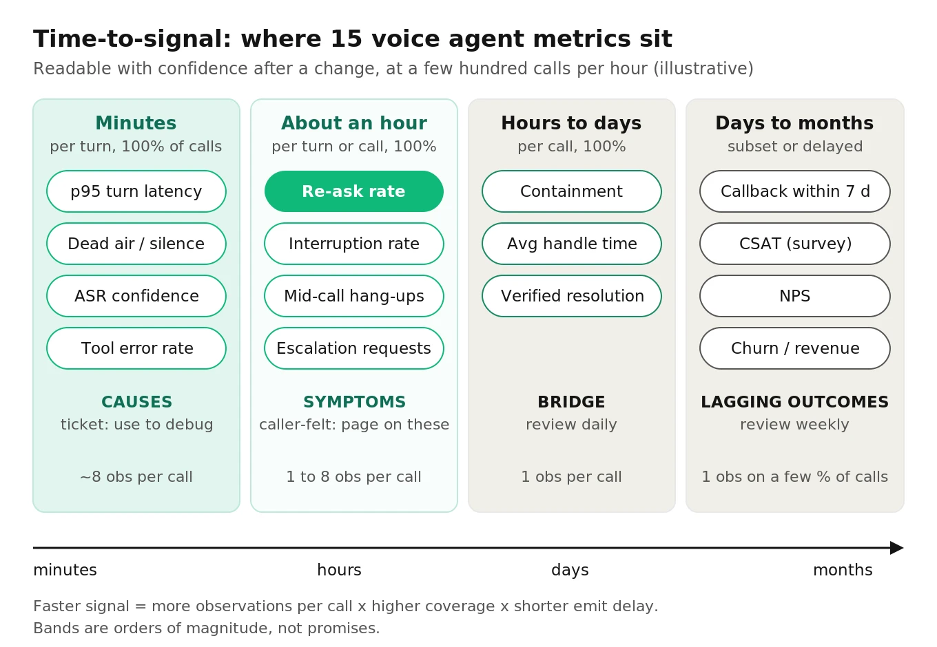
Three things in this map are less obvious than they look.
Rows 1 to 4 are mostly causes; rows 5 to 8 are symptoms. Latency and tool errors explain why a call went wrong. Re-asks, interruptions and hang-ups are what the caller actually experiences. Google's SRE guidance makes the same split for servers: pages should fire on symptoms users feel and causes should help you debug (Monitoring Distributed Systems). In a voice agent, turn-level symptoms are both fast and caller-felt, which is unusual and useful. They are the best paging candidates you have. For what each symptom costs, see interruption rate, silence rate and the cost of latency.
Containment is a bridge, not a lagging truth. It is fast enough to watch daily, but it is measured at hang-up, before you know whether the caller's problem was actually solved. A call that "contained" and then called back on Thursday was a failure. That is why rows 11 and 12 exist. For the distinction, see first contact resolution.
Re-ask rate is the most underused metric on the list. It captures STT errors, bad audio, confusing prompts and repetition loops in a single number, it is cheap to compute from transcripts, and it sits right where a caller's patience starts to drain. Repetition loops are its extreme form.
Defining re-ask rate so it is computable
Re-ask rate = (agent turns that ask the caller to repeat or rephrase + caller turns that repeat the previous caller turn) / agent turns. A simple detector is enough to start:
# Illustrative re-ask detector. Version the patterns: prompt changes can shift them.
import re
from difflib import SequenceMatcher

AGENT_REASK = re.compile(
    r"\b(sorry|pardon|didn'?t (catch|get) that|could you (repeat|say that again)|"
    r"one more time|can you spell)\b", re.I)

def count_reasks(turns):
    """turns: list of {"role": "agent"|"user", "text": str}, in call order."""
    reasks, last_user = 0, None
    for t in turns:
        if t["role"] == "agent" and AGENT_REASK.search(t["text"]):
            reasks += 1                       # agent asked the caller to repeat
        elif t["role"] == "user":
            if last_user and SequenceMatcher(None, last_user.lower(),
                                             t["text"].lower()).ratio() > 0.8:
                reasks += 1                   # caller repeated themselves
            last_user = t["text"]
    return reasks
Regex misses paraphrases ("let me make sure I have that right" is sometimes a re-ask and sometimes good practice). Once the metric matters, swap the pattern match for a classifier that answers one yes/no question per turn. Keep a hand-labeled set of 200 turns to check it against.
What the research says about predicting satisfaction
Dialogue-systems research worked on this for decades before LLM agents. Three findings carry over.
Satisfaction can be modeled from task success plus interaction costs. The PARADISE framework (Walker et al., ACL 1997) treats user satisfaction as the target. It fits a regression on task success and per-dialogue "costs" such as number of turns and repair utterances. The repair terms are re-asks in today's language. A follow-up study applied the method to three spoken dialogue systems and reported that the models generalized across systems, conditions and user populations (Walker, Kamm and Litman, 2000). The practical lesson: your leading metrics belong on the right-hand side of a regression whose left-hand side is CSAT. They should not be eyeballed one at a time.
Turn-level quality tracks end-of-call satisfaction, but visible emotion does not. Schmitt and Ultes built Interaction Quality, an exchange-level score that can be computed at any point in a call. On the CMU Let's Go bus system, expert IQ ratings correlated with real user satisfaction at ρ = .66. Their model predicted user satisfaction at ρ = .74 on lab data. A manually labeled negative-emotion feature added only a marginal gain, and the authors note that only a minority of users show visible anger when they are dissatisfied (Speech Communication, 2015). For you, that means a sentiment score is a weak early-warning metric. Interaction features like repairs and timing carry more of the signal.
Several weak proxies combined beat any single one. Athey, Chetty, Imbens and Kang formalized the "surrogate index": predict the long-term outcome from several short-term outcomes and use that prediction as the metric (arXiv 1603.09326). In their job-training application, short-term outcomes from the first 1.5 years recovered the 9-year effect, with standard errors 35% smaller. The key assumption is that the long-term outcome is independent of the change once you condition on the surrogates. In voice terms, a regression that damages CSAT through a path none of your leading metrics see stays invisible. Example: the agent fluently states the wrong refund policy. Re-asks, latency and interruptions all look fine, and the caller calls back angry on Friday.
Two results from online experimentation complete the picture. Google's "Focusing on the Long-term" paper showed that short-term metrics can point the wrong way on long-term user behavior. The authors built a model that predicts long-term effects from short-term metrics (Hohnhold, O'Brien and Tang, KDD 2015). Deng and Shi at Microsoft framed good metrics as having two properties: sensitivity (does it move detectably?) and directionality (does it move in the same direction as the long-term outcome?) (KDD 2016). Every leading metric you adopt needs evidence on both.
Proving a leading metric predicts the lagging one
There are four tests, in order of strength. Run all four before you let a metric page anyone.
Test 1: Call-level linkage (strongest, cheapest)
Every surveyed call also has a re-ask count, a p95 latency and a tool error count. Join them. Compare CSAT for calls with and without the leading event, then fit a logistic regression with controls such as day of week, flow and caller type. This uses the actual causal unit, the call, and it needs no time-series assumptions. A few weeks of survey responses is usually enough.
Test 2: Lagged correlation on daily series
Aggregate the leading metric by day and the lagging metric by day, then correlate the leading metric at day t with the lagging metric at day t+k for k = 0 to 7. Two traps live here.
- Pick the right date column. If you bucket CSAT by the day the call happened, the correlation peaks at lag 0, because both metrics describe the same calls. If you bucket by the day the survey arrived, which is what most dashboards show, the peak shifts by the reporting delay. The first view tells you whether the link exists. The second tells you how much warning you get. Compute both.
- Remove shared trends first. Two series that both drift (traffic growth, a seasonal caller mix) correlate at every lag for no causal reason. The standard fix is prewhitening, or at least differencing (Penn State STAT 510, Lesson 9.1). For call data, a 7-day difference also removes the weekly cycle.
Test 3: Granger-style check
Ask whether past values of the leading metric improve a forecast of the lagging metric beyond the lagging metric's own past. statsmodels' `grangercausalitytests` tests whether the series in the second column Granger-causes the series in the first (docs). Getting the column order wrong is the most common mistake. "Granger causes" means "helps predict". It does not mean "causes". A deploy that moves both metrics at once will pass.
Test 4: Directionality on known incidents
List every regression and every improvement you shipped in the past six months. For each one, check whether the leading metric moved first and in the expected direction. A metric that moved the right way in 5 of 6 known events is worth more than any p-value. This is Deng and Shi's directionality test using your own history.
Sample size for the validation itself
A daily-series correlation needs more days than people expect. Using the Fisher z approximation, `n ≈ ((z_α/2 + z_β) / atanh(r))² + 3`. At α = 0.05 and 80% power:
| True correlation r | Days of data needed |
|---|---|
| 0.5 | about 29 |
| 0.4 | about 47 |
| 0.3 | about 85 |
So three months of daily data detects only moderate correlations. That is the strongest argument for Test 1. Call-level linkage gets thousands of observations in the time a daily series gets dozens.
Runnable-shaped pandas code
This assumes one row per call with turn counts and an optional survey response. It runs as written against a CSV with these columns (simplified).
import pandas as pd
import statsmodels.formula.api as smf
from statsmodels.tsa.stattools import grangercausalitytests

# columns: call_id, started_at, n_agent_turns, n_reask_turns, csat (1-5 or blank),
#          csat_submitted_at (blank if no response)
calls = pd.read_csv("calls.csv", parse_dates=["started_at", "csat_submitted_at"])
calls["top2"] = (calls["csat"] >= 4).astype(float).where(calls["csat"].notna())

# Leading: re-ask rate per agent turn, bucketed by the day the CALL happened
lead = calls.set_index("started_at").resample("D")[["n_reask_turns", "n_agent_turns"]].sum()
lead["reask_rate"] = lead["n_reask_turns"] / lead["n_agent_turns"]

# Lagging, two views: by call day (does a link exist?) and by survey-arrival day
# (how much warning does the dashboard get?)
surveyed = calls.dropna(subset=["top2"])
csat_by_call = surveyed.set_index("started_at").resample("D")["top2"].mean()
csat_by_arrival = surveyed.set_index("csat_submitted_at").resample("D")["top2"].mean()

def lagged_corr(x, y, max_lag=7, season=7):
    """corr(x_t, y_{t+k}) for k = 0..max_lag after a weekly difference."""
    xd, yd = x.diff(season), y.diff(season)
    return pd.Series({k: xd.corr(yd.shift(-k)) for k in range(max_lag + 1)})

print(lagged_corr(lead["reask_rate"], csat_by_call).round(2))
print(lagged_corr(lead["reask_rate"], csat_by_arrival).round(2))

# Granger-style check. Column order is [effect, candidate cause].
df = pd.concat({"csat": csat_by_arrival, "reask": lead["reask_rate"]}, axis=1)
df = df.diff(7).dropna()
res = grangercausalitytests(df[["csat", "reask"]], maxlag=3)
for lag, (tests, _) in res.items():
    print(f"lag {lag}: p = {tests['ssr_ftest'][1]:.4f}")

# Call-level linkage: the strongest and cheapest evidence
surveyed = surveyed.assign(
    had_reask=(surveyed["n_reask_turns"] > 0).astype(int),
    dow=surveyed["started_at"].dt.dayofweek)
print(surveyed.groupby("had_reask")["top2"].agg(["mean", "count"]))
fit = smf.logit("top2 ~ had_reask + C(dow)", data=surveyed).fit(disp=0)
print("re-ask coefficient:", fit.params["had_reask"], "p:", fit.pvalues["had_reask"])
Generate a synthetic table with a built-in per-call effect of re-asks on CSAT plus a slow shared trend, and this script typically shows an obvious call-level gap, weak lagged correlations smeared across every lag, and a Granger test that misses significance. Real links often look weak in daily aggregates. Do not drop a metric because Test 2 or Test 3 is inconclusive if Test 1 and Test 4 are strong.
Once two or three leading metrics pass, combine them. Fit the call-level model with all of them, score every call with it, and plot that "predicted CSAT" next to survey CSAT. That is a surrogate index with 100% coverage and minute-level freshness. Where it disagrees with the survey, the disagreement points at a failure path your leading metrics do not see.
Lead time math: how much warning you actually get
Lead time is the difference between two times-to-signal:
`lead_time = time_to_signal(lagging) − time_to_signal(leading)`
and the damage a regression does is roughly:
`affected_calls ≈ call_rate × (time_to_signal + time_to_mitigate)`
Here are the numbers for an illustrative deployment. Every value is an assumption you should replace with your own: 3,000 calls a day, about 200 an hour at peak, 8 agent turns per call, an 8% survey response rate, and a baseline where 20% of calls contain at least one re-ask.
Re-ask rate, call level. To detect a rise from 20% to 28% of calls (one-sample test, α = 0.05, 80% power): `n = (z_α/2·√(p₀q₀) + z_β·√(p₁q₁))² / (p₁ − p₀)²` ≈ 211 calls. At 200 calls an hour, that is about 63 minutes.
Re-ask rate, turn level. From 5% to 8% of turns, the same formula gives about 477 turns. Turns in the same call are correlated, so apply a design effect, about 2 as a working assumption. That gives roughly 950 turns, or about 120 calls, which is about 36 minutes. Turn-level metrics are faster as long as you account for the clustering.
CSAT. For top-2-box CSAT to drop from 80% to 75%, the same formula needs about 528 responses. At 8% response on 3,000 calls, you get 240 a day, so you need about 2.2 days of responses plus the time it takes callers to answer. For a 3-point drop, 80% to 77%, you need about 1,440 responses, or 6 days.
Callback within 7 days. You need at least 7 days just for the window to close on Monday's calls, plus volume.
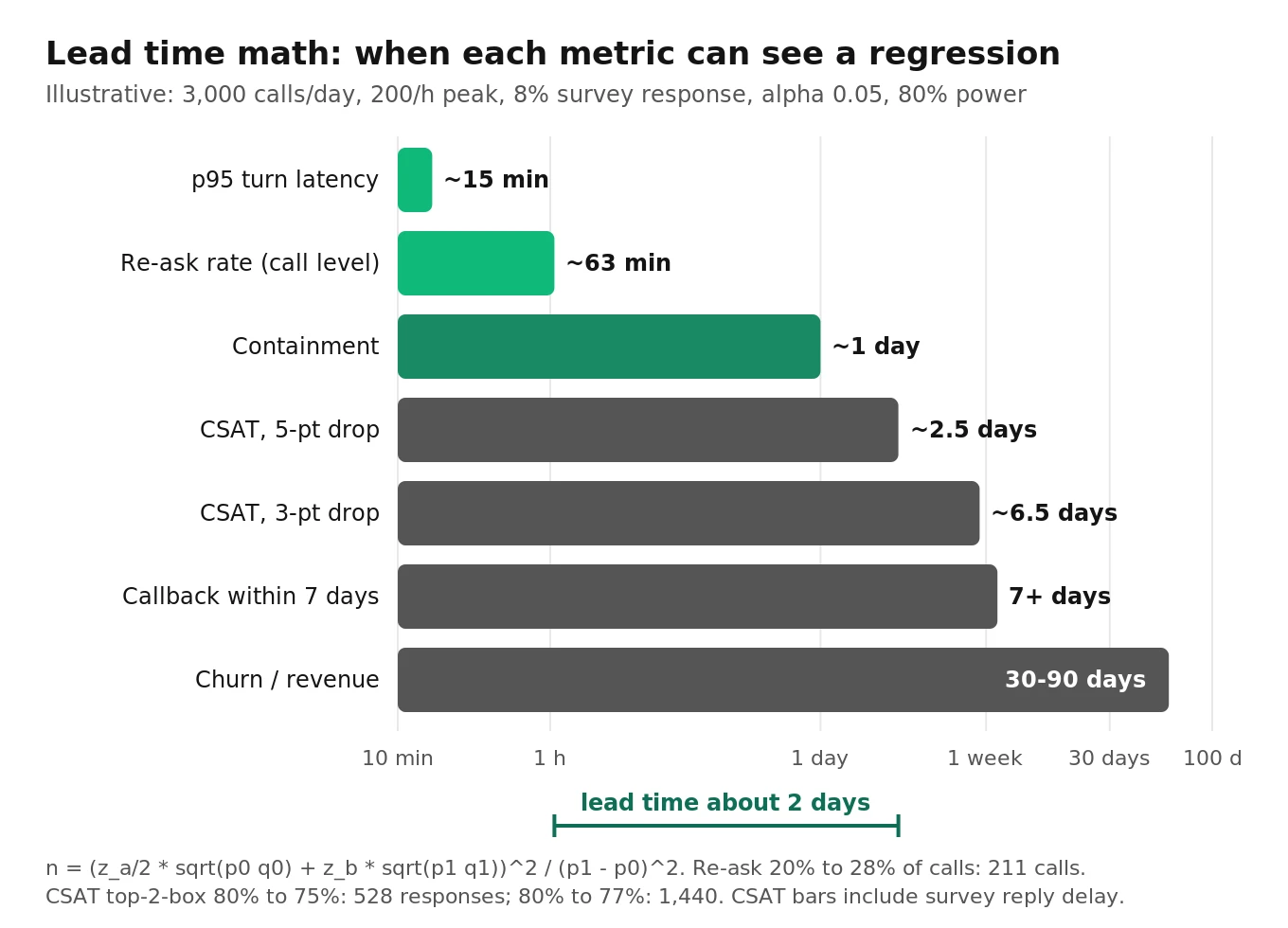
So in this example a re-ask alert gives about 2 days of lead over CSAT for a 5-point drop and about 6 days for a 3-point drop. With a weekly review and no alerts, the regression runs a full week: about 21,000 affected calls. With a leading alert and a 30-minute rollback, it runs about 1.5 hours: about 300 calls. The arithmetic is simple; the hard part is having turn-level data.
Alert design: leading metrics page, lagging metrics get reviewed
The rule of thumb: alert on what is fast and caller-felt, review what is slow and decisive. Never page on CSAT. The sample is too small and too late, and a pager that fires on noise trains people to ignore it.
| Tier | Metrics | Window | Fires when | Route |
|---|---|---|---|---|
| Page | re-ask rate, dead-air rate, mid-call hang-up rate, tool error rate | 5 min AND 1 h | both windows above baseline × factor, per flow and version | on-call, with rollback link |
| Ticket | p95 turn latency, ASR confidence, interruption rate, escalation requests | 1 h AND 6 h | sustained shift past control limits | owning engineer, same day |
| Daily review | containment, AHT, verified resolution | day vs same weekday last 4 weeks | outside control band | standup |
| Weekly review | CSAT, callback within 7 days, NPS, churn | week, cohorted by call date | trend or gap vs predicted CSAT | product + ops |
Borrow the multiwindow structure, not the numbers. The Google SRE workbook's multiwindow, multi-burn-rate alert pages when the error-budget burn rate exceeds a threshold over both a long window and a short one. Its recommended page is a burn rate of 14.4 over 1 hour and 5 minutes, which equals spending 2% of a 30-day budget in an hour (Alerting on SLOs). The long window gives significance, and the short window makes the alert stop firing quickly after a rollback. The 14.4 does not transfer. That number assumes errors are rare. A 5% baseline re-ask rate times 14.4 is 72%, a level you will never see. For turn-level voice metrics, set the factor from the sample-size math above, typically 1.3× to 1.6× baseline. Then require the 1-hour window to contain at least the n you computed. Threshold mechanics are covered in depth in setting production thresholds and slow drift in detecting metric drift. This section is only about which tier a metric belongs in.
Segment before you threshold. A regression in your ordering flow gets diluted by unaffected billing calls in a global rate. Compute every paging metric per flow, per `agent_version`, and per provider (STT, TTS, LLM, carrier). Most of the time the version split is the root-cause analysis.
Gotchas that make leading metrics lie
- ASR confidence is not comparable across models. Switching STT models or versions shifts the whole confidence distribution, even when accuracy is unchanged. Reset the baseline at every model change, or the "drop" you see is just calibration. Audio path issues show up here too; see phone audio quality.
- Interruption rate can fall when things get worse. Callers who have given up stop barging in, and a longer endpointing timeout suppresses barge-ins while adding latency. Check the sign of the relationship with Test 4. Do not assume it.
- Recent days of callback-within-7-days always look good. Calls from the past 7 days have not finished their window, so their callback rate is understated. This is right-censoring. Grey out incomplete days or plot only closed cohorts.
- CSAT can rise during a regression. If the survey is offered only after contained calls, or angry callers hang up before it plays, the respondent pool shifts. Track response rate alongside CSAT. A falling response rate with flat CSAT is a warning.
- Prompt changes move detectors. A new prompt that confirms every address with "sorry, let me read that back" inflates regex re-ask counts with no caller impact. Version the detector together with the prompt.
Worked example: re-ask rate catches a regression 2 days before CSAT
This is an illustrative scenario with the same assumed volumes as above. It is not a customer case.
Setup. A restaurant group runs an in-house order-taking agent on Pipecat with streaming STT, an LLM and TTS over Twilio SIP. Normal traffic is 3,000 calls a day. The baseline re-ask rate is 5% of agent turns, and 20% of calls have at least one re-ask. Top-2-box CSAT is 80% at an 8% response rate.
Monday 10:00. A config refactor ships. It accidentally drops the STT custom-vocabulary list that held menu item names. Generic words still transcribe fine, but "birria quesatacos" now comes out as three unrelated words. Latency is unchanged, tool errors are unchanged, and nothing crashes.
Monday 10:05 to 11:05. In the ordering flow, the agent starts asking callers to repeat item names, and callers repeat themselves. Re-ask rate rises to 8% of turns, and 28% of calls now have a re-ask. ASR confidence on user turns dips slightly, which is ticket-tier and easy to miss. Interruption rate barely moves.
Monday 11:05. The page fires. The 1-hour window holds about 200 ordering-flow calls at 1.6× baseline re-ask, and the 5-minute window agrees. The alert links to the version split: all of the excess is on the new `agent_version`.
Monday 11:35. Rollback. The 5-minute window drops below threshold, and the page resolves within minutes. About 300 calls were affected.
The counterfactual. Suppose there were no leading alert. Monday's survey responses come in through Monday night and Tuesday, and daily CSAT looks noisy, not alarming. Detecting a 5-point drop needs about 528 responses, so CSAT becomes statistically readable around Wednesday afternoon. If the weekly review is on Monday, the real discovery is a week later, and about 21,000 calls are affected. The callback-within-7-days metric confirms it the following week, after the damage is done.
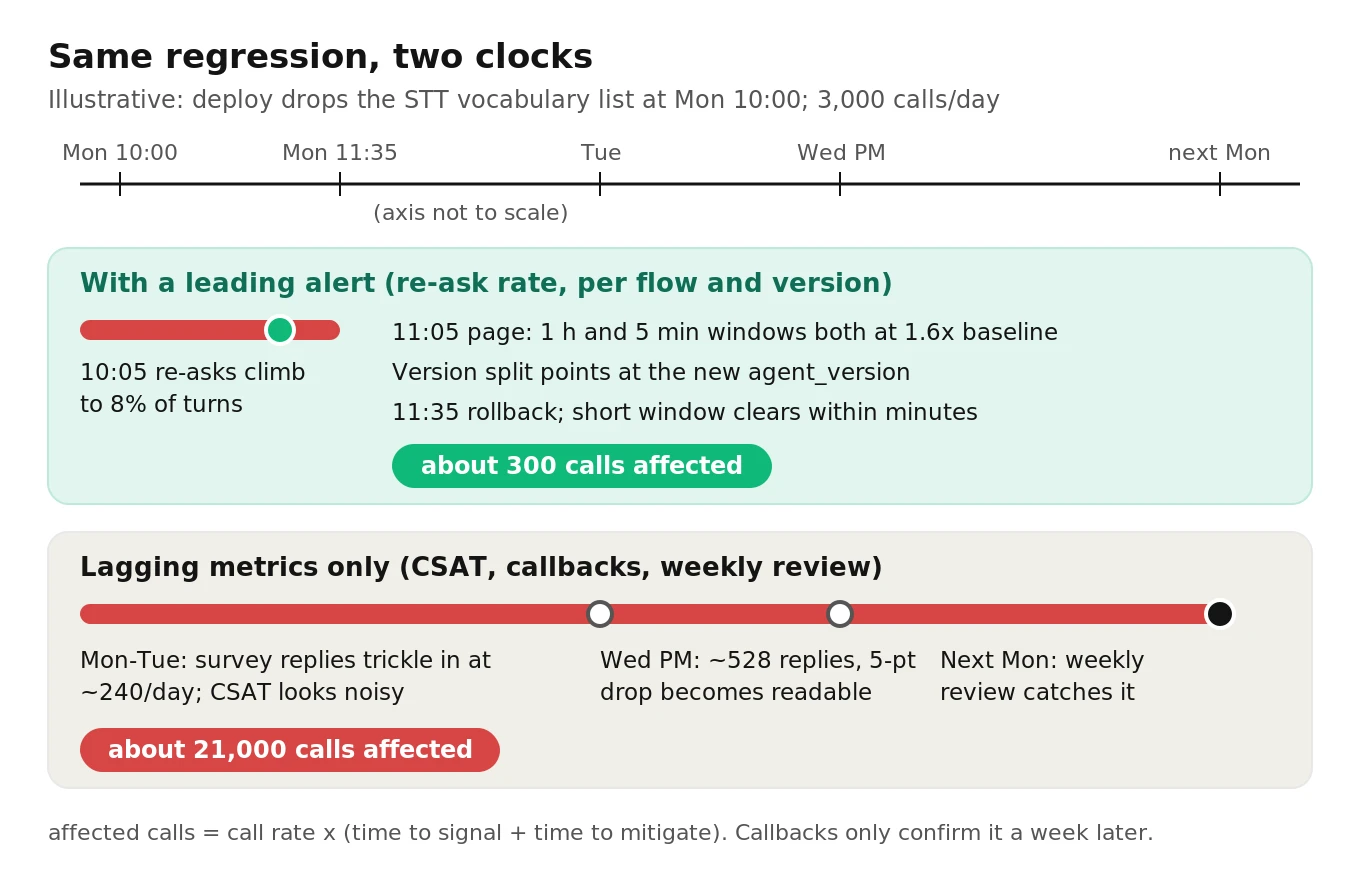
Two details make this example work. First, the alert was per flow. Billing calls do not use menu vocabulary, so a global re-ask rate would have moved about half as much. Second, the team had already validated re-ask against CSAT with call-level linkage. So the on-call engineer trusted the page instead of waiting for "real" numbers.
Dashboard layout: three rows on three clocks
Lay out the dashboard by clock speed so nobody compares a 5-minute number with a weekly one. The full tile-by-tile design is covered in the voice agent KPI dashboard guide, and the metrics scorecard covers release judgment. The leading/lagging layer adds this structure:
| Row | Refresh | Tiles | Split by |
|---|---|---|---|
| 1. Live leading | 1 to 5 min | re-ask rate, dead-air rate, p95 turn latency, tool error rate, mid-call hang-ups | flow, agent_version, provider |
| 2. Daily bridge | hourly to daily | containment, escalation requests, AHT, verified resolution, predicted CSAT (surrogate) | flow, version |
| 3. Weekly lagging | daily refresh, weekly read | survey CSAT plus response rate, callback within 7 days (closed cohorts only), NPS, churn | cohort by call week |
Add two panels most teams forget:
- Predicted vs actual CSAT. This puts the surrogate index from your leading metrics next to survey CSAT, cohorted by call date. A widening gap means a failure path your leading metrics cannot see. That gap is your cue to add a metric.
- Deploy markers on every row. Vertical lines for prompt, model, provider and config changes. Most "mysterious" shifts line up with one.
For more on why survey CSAT behaves the way it does, see measuring CSAT for voice agents.
How to set up leading and lagging indicators for your voice agent
1. Log at turn level. For every turn, record the timestamps for end of user speech, first agent audio, any barge-in, and tool call start and end with status. Add transcript text with role, ASR confidence, and `agent_version` and provider IDs. Without turn data you have no leading metrics.
2. Compute the six core leading metrics per call. These are re-ask count, dead-air seconds, p95 turn latency, tool error count, interruption count, and hung-up-mid-turn. Store them on the call row next to the outcome fields.
3. Define the lagging outcomes precisely. Write down CSAT definitions (top-2-box, scale, when the survey is offered), callback window and matching key (phone number, account ID), and resolution criteria. Cohort all of them by call date.
4. Run the four validation tests. Do call-level linkage, lagged correlation on both date views after a 7-day difference, a Granger check with the column order right, and directionality on past incidents. Keep only metrics that pass Test 1 and Test 4.
5. Size your windows from the math. For each paging metric, compute the n needed to detect the shift you care about. Set the long window so it holds that n at normal peak traffic, and set the short window at 5 minutes.
6. Tier the alerts. Paging goes to fast, caller-felt, validated metrics, per flow and version. Tickets go to causes. Bridge metrics get a daily review. Lagging outcomes get a weekly review against predicted CSAT.
7. Fit a surrogate index. Regress call-level CSAT on the validated leading metrics, score every call, and chart predicted against actual. Refit quarterly and after major model changes.
8. Test before live callers, then rehearse. Replay a fixed scenario suite against every release candidate and compare leading metrics to the previous version. This shows most regressions before production does. Then inject a known regression, such as removing a vocabulary list in staging, and confirm the page fires within the window you computed. Independent evaluation fits here. A third party like Evalgent can run the scenario suite on every release and score verified resolution, the one outcome a team should not grade for itself, so your leading metrics are validated against ground truth instead of your own judgment.
Frequently asked questions
What is the difference between leading and lagging indicators for a voice agent?
Leading indicators are signals you can read within minutes or hours on every call, such as re-ask rate, dead air, p95 turn latency and tool errors. Lagging indicators are outcomes like CSAT, callbacks and churn. They take days or weeks to read and often cover only a fraction of calls. Leading metrics warn you; lagging metrics confirm the business impact.
Which voice agent metrics best predict CSAT?
Interaction-cost metrics usually work best: re-ask or repair rate, dead air, turn latency and mid-call hang-ups, plus verified task success. Research on spoken dialogue systems found that repairs and task success predict satisfaction, while visible negative emotion added little. Validate on your own calls with call-level linkage before trusting any of them.
Should I set alerts on CSAT?
No. Survey CSAT arrives late and on few calls. In the illustrative example above, a 5-point drop needed about 2 days of responses to detect, and a 3-point drop needed about 6. Paging on it creates noisy alerts that people learn to ignore. Review CSAT weekly, cohorted by call date, next to a predicted CSAT built from leading metrics.
How do I validate that a leading metric actually predicts a lagging one?
Run four tests. First, join leading metrics to surveyed calls and compare outcomes. Second, compute lagged correlation on differenced daily series. Third, run a Granger-style test. Fourth, check directionality on past incidents. Call-level linkage and incident directionality are the most reliable. Daily correlations need roughly 47 days of data to detect a correlation of 0.4.
What is time-to-signal?
Time-to-signal is how long after a change you can confidently tell that a metric moved. It equals emit delay plus pipeline delay plus accumulation time. Accumulation time is the required sample size divided by observations per hour, and it usually dominates. Per-turn metrics on every call accumulate evidence far faster than survey metrics on a few percent of calls.
Is containment rate a leading or lagging indicator?
It sits in between. Containment is measured at hang-up on every call, so it is readable within hours. But it does not tell you whether the problem was actually solved. A contained call followed by a callback is a failure. Treat containment as a daily bridge metric and confirm it with verified resolution and callback within 7 days.
Why does my callback rate look better for the most recent week?
That is right-censoring. Calls from the last 7 days have not finished their callback window yet, so their rate is understated. Show only closed cohorts or grey out incomplete days. Any windowed lagging metric, including churn, has the same artifact.
Can I use Google SRE burn-rate alerts for voice agent metrics?
Use the structure, not the numbers. The multiwindow approach is useful: page only when a long and a short window both exceed the threshold. But the 14.4 burn-rate figure assumes rare errors. For voice metrics with baselines like 5%, size the threshold factor and the long window from a sample-size calculation instead.
The bottom line
Leading vs lagging indicators come down to a clock: re-ask rate, dead air, latency and tool errors tell you within an hour what CSAT and callbacks confirm days later. Validate the link with call-level data, page on the fast metrics per flow and version, and review the slow ones weekly against a predicted CSAT, so the next bad deploy affects hundreds of calls, not tens of thousands.
Related Articles
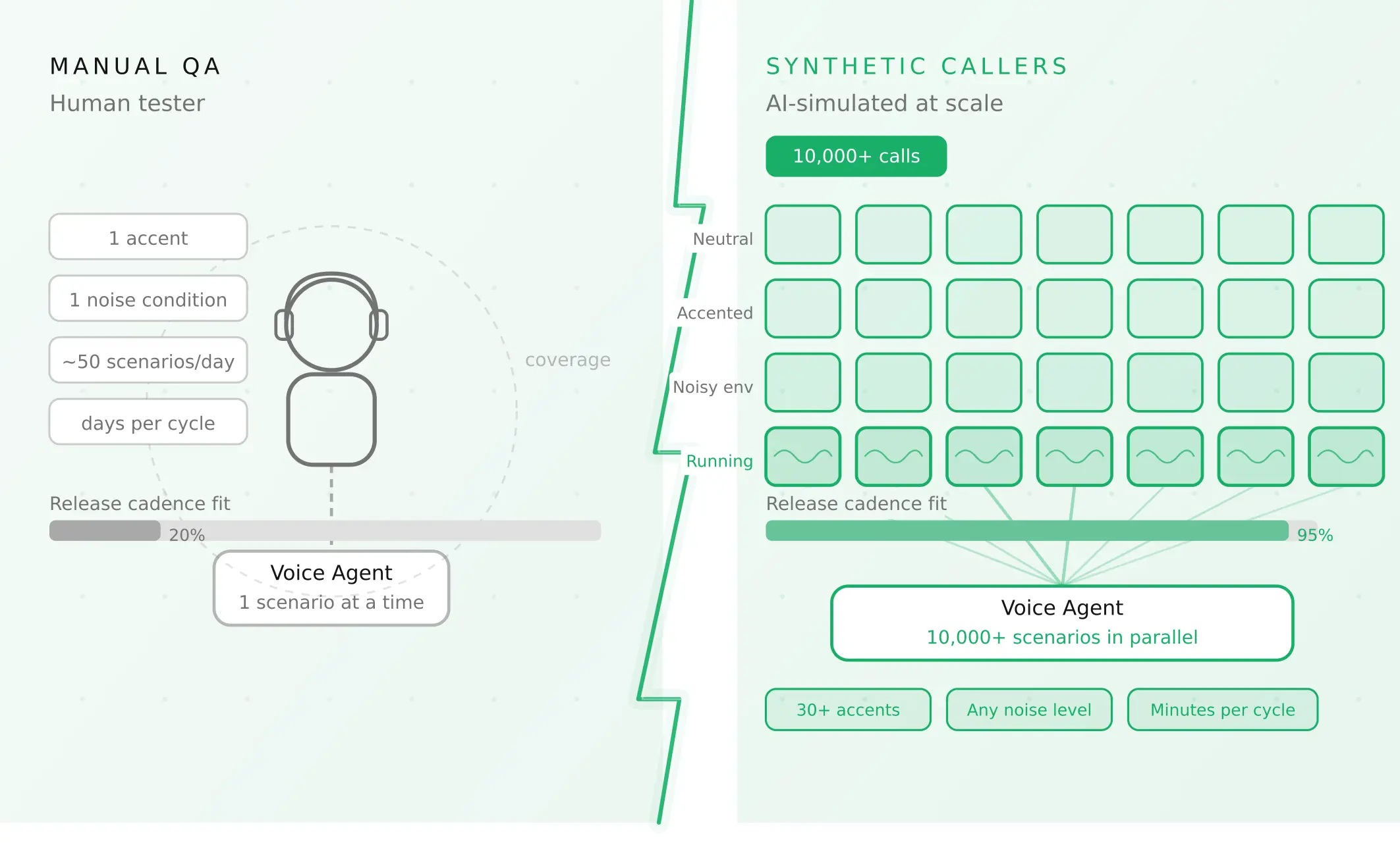
How to automate voice agent testing: synthetic callers vs manual QA
Learn how ai test automation replaces manual QA for voice agents. Compare synthetic callers vs human testers, with a 5-step framework to scale without hiring.
Read more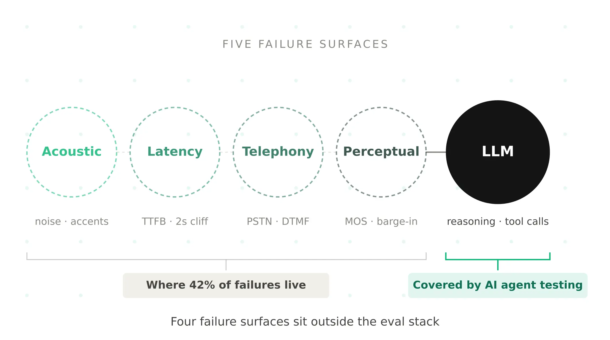
AI Agent Testing vs Voice Agent Testing: What General Tools Miss for Voice
AI agent testing measures text outputs. Voice agent testing measures behaviour through an acoustic pipeline. Five failure categories general tools miss.
Read more